Beyond Leave Tables: A State-of-the-Art CNN Static Evaluator for Scrabble
In 2022 I built my own computer. One of my main desires for the computer was to be able to add a graphics card to it - not to play games, since I mostly just play games on the Nintendo Switch (2) - but for doing Scrabble-related computational tasks. My job at the time was as a data engineer at a recently acquired telephony startup. We used neural networks a bunch, and I’d learned a bit about training them, but I was mostly on the data side – building training data pipelines, serving neural networks in production, and so on. In college (many years ago) I took a class on neural networks where we actually implemented the entire perceptron + backpropagation, etc algorithms ourselves. But neural networks were mostly seen as a curiosity back then. They were good at detecting handwritten digits, but nothing too much more complex than that. But in recent years, large amounts of data, better gradient functions, faster hardware, more regularization tricks, better software, and so on turned neural networks from a neat toy for digit recognition to a default method for perception, language, game-playing, drug discovery, and more - all within the last 15 years or so.
Still, it took me a while to get the confidence to try training a neural network to play Scrabble, since I don’t actually know how to use all these new tricks. I played around with Keras and Pytorch a bit to build really simple models, read the AlphaGo paper, and so on, so I know very roughly what is required. But in recent years, another recent invention has taken the world by storm - Generative AI. At work we’ve been using ChatGPT o3 as well as Cline and other agentic coding tools, and they’re astonishing and rapidly improving. So a few weeks ago I kicked off a conversation with o3 about how to build a neural network model for Scrabble. Over a few days I would ask it if it’s considered this or that, and while there were some occasional hallucinations (it kept insisting that Scrabble neural networks had beaten Quackle’s championship player by this many ppg and so forth), it was helpful that I already know how to code and have basic knowledge of neural networks.
So we prototyped a model together. The idea is largely based on what AlphaGo did - a convolutional neural network for the board plus additional other features. The next few paragraphs will be pretty technical, but this blog also serves as documentation for trying to reproduce this in the future.
ConvNet section - architecture, datastream, and training loop
(A plain-English walk-through of the code above so future-me doesn’t have to squint at it again.)
Data generation
Data is generated by the Macondo autoplay command. Autoplay pits two bots against each other. Running two instances of the default static bot (HastyBot - our fast static evaluator) processes about 1,000 games per second on my computer. It’s fast, but it still takes a few hours to collect a few million games.
Games are logged one turn at a time (interleaved, since the game runner is multithreaded). The main parameters are the player on turn’s rack, their play, leave, and score. Each game can be reproduced from this log.
Feature tensor
| Piece | Shape | Count | Notes |
|---|---|---|---|
| Board planes | 85 × 15 × 15 |
18 900 floats | one-hot layers for every letter & premium, plus masks for cross-checks, uncovered bonus squares, etc. |
| Scalar vector | 76 |
76 floats | bag counts, score, power-tile flags, leave value, … |
| Target | 1 |
single float | tanh-squashed final prediction (≈ −1 … +1). |
The feature tensor is generated by a Go script which plays through all the turns in sequence, keeping track of an internal map of active games, and freeing memory when needed. The large majority of the tensor is 85 15x15 representations of a Scrabble board:
- 26 15x15 matrices, one for each letter on the board, using one-hot encoding. For example, the matrix for the letter
Owill have a1.0in every position where there is an O, and a 0.0 otherwise. So many of these matrices are very sparse. This is good for a neural network. - 1 15x15 matrix for whether the tile on this position is a blank or not.
- 26 15x15 matrices for all the horizontal cross-sets (whether each letter can be placed on this square to form a horizontal word)
- 26 15x15 matrices for all the vertical cross-sets
- 4 15x15 matrices for all empty bonus squares (2L, 3L, 2W, 3W)
- Our opponent’s last play (1.0 for all squares where they last played their tile)
- Our current play - the one we are trying to evaluate
The scalar vector is then:
- 27 scalars representing our rack. Everything is normalized to a [0, 1] range by dividing the count of tiles by 7.
- 27 scalars representing the bag. We divide by the total number of tiles in the bag for each scalar. This not only normalizes to a [0, 1] range, but also encodes the rough probability of drawing that tile out of the bag.
- 8 scalars for “last move was exchange”. The first scalar is a 1.0 if it was an exchange, and the next 7 are basically a one-hot encoding of how many tiles were actually exchanged.
- 6 scalars for power tiles. One for each of JQXZ?S, and the value is normalized to [0, 1] by dividing by the count of that tile in the distribution.
- 2 scalars for vowel/consonant ratio in the bag (divide V/C by number of tiles in the bag)
- 2 scalars for vowel/consonant ratio in our rack
And for the final even juicier parameters:
- 1 scalar for our move score (the one we are evaluating)
- 1 scalar for our leave value
- 1 scalar for number of tiles in bag divided by 100
- 1 scalar for the spread of this position (our score minus theirs)
Note that the tensor here has the play we are trying to evaluate already placed on the board. All cross-checks, leave values, bag contents, etc. assume that the play has just been placed, but we haven’t yet drawn replacement tiles.
The scalars for move scores, spreads, and leaves were all normalized to a [-1, 1] range with the very commonly used in machine learning hyperbolic tangent function (TANH#).
A training “frame” is therefore (18 977 + 1) × 4 bytes ≈ 76 kB. The helper script on the data-generation side writes each frame as
[ 4-byte little-endian length | raw bytes ]
which lets the trainer treat stdin as an endless binary stream.
Game assembler
The game assembler takes in as input the log file from the Macondo autoplay command, and outputs a binary stream of data in the format above. It “assembles” games together one turn at a time in memory, using the Macondo engine itself to implement the rules of Scrabble. It will also randomly transpose half the games to make sure our network isn’t biased (This is for you verties out there!)
When the assembler has enough data for a game, it begins outputting one ML vector per turn. On my computer it outputs around 1 GiB of ML vectors per second.
Trainer
The training code is a few hundred lines of Python PyTorch code. It listens on this binary data stream.
-
The producer thread sits on
sys.stdin.buffer, peels off len + payload pairs, and pushes them into two multiprocessing.Queues:-
the first val_q gets the first VAL_SIZE = 150 000 frames (one-shot validation set);
-
the rest go to train_q. A sentinel None is en-queued when EOF is reached so the workers can shut down cleanly.
-
-
QueueDataset turns each queue into an IterableDataset that yields
(board, scalars, target)tensors on demand. -
DataLoader pulls from train_q with
num_workers = os.cpu_count()and batches tobatch_size = 2 048. Because everything is streamed, RAM usage stays ≈ batch-size × tensor-size (a few hundred MB even on CPU boxes). Training on the actual raw positional data (without generating it on the fly) would mean over a terabyte of vectors for just a few million games!
Network architecture
Input (85×15×15)
│
├─ Conv3×3, 64ch  + BN + ReLU
│
├─ 6 × { Conv3×3 + BN + ReLU  →  Conv3×3 + BN  →  residual add + ReLU }
│     (Residual blocks identical to those in AlphaGo Zero, width 64)
│
├─ Global-Average-Pooling → 64-d vector
│
├─ Concat(64-d, 76-d scalar features) → 140-d
│
├─ FC-128  + ReLU
│
└─ FC-1   →  tanh  →  **value ∈ (−1, 1)**
Why this shape?
-
A thin (64-filter) conv trunk is plenty for 15×15 boards. We can consider going wider to see if it helps some more.
-
Global-average pooling collapses spatial info and lets the head stay invariant to board translations. It converts location-specific activations into board-level cues.
-
Concatenating the hand-crafted scalar vector late keeps the conv stack “vision-only” and lets the multilayer perceptron (MLP) reason about bag/timeline meta-info.
The target
There are many choices for what you should train the network to predict. The most obvious one is just win. I ended up choosing this - whether the game ends up in a win or loss. I mapped win to +1.0, loss to -1.0, and draw to 0.0, and set this as the network’s one prediction. I’ll talk more about other things I tried later in this post.
Training recipe
| Hyper-param | Value | Rationale |
|---|---|---|
| Optimiser | AdamW (lr 3 e-4, wd 1 e-4) |
stable on mixed precision, good default for tabular + vision mixes. (Might still want to play more with learning rate) |
| Loss | SmoothL1 |
ChatGPT told me |
| Batch size | 2 048 | fits on my 8GB graphics card (NVIDIA GeForce RTX 3070 Ti) |
| Mixed precision | torch.autocast + GradScaler |
~2× throughput on GPU/MPS. |
| Validation cadence | every 500 steps (~1 M positions) | keeps wall-clock < 5 s/val pass. |
| Early-best checkpoint | overwrite best.pt whenever val loss improves |
so long overnight runs always leave a usable model. |
When I got my graphics card I was satisfied with 8 GB VRAM, but very soon after, LLMs started becoming a thing, and many don’t fit in my little card anymore. (Not that this is an LLM project). Still, a batch size of 2048 easily fits in my graphics card. The card has no trouble with training; the biggest bottleneck is actually in my game assembler, which has to play every game a turn at a time, compute the cross-sets, allocate the vector, and so forth. It’s written in Go, which is a good, fast language, but rewriting this in something like C (and making it more optimized) would greatly increase training speed.
As it is, I can still train at around 10K positions per second. This means for a data set with about 7.5M games, we can train a model in about 4 to 5 hours.
Every 1 million positions or so, we re-run a validation set. If the validation loss is better than the last validation loss, it creates a new model checkpoint. The curve below shows our best-performing model’s loss curve.
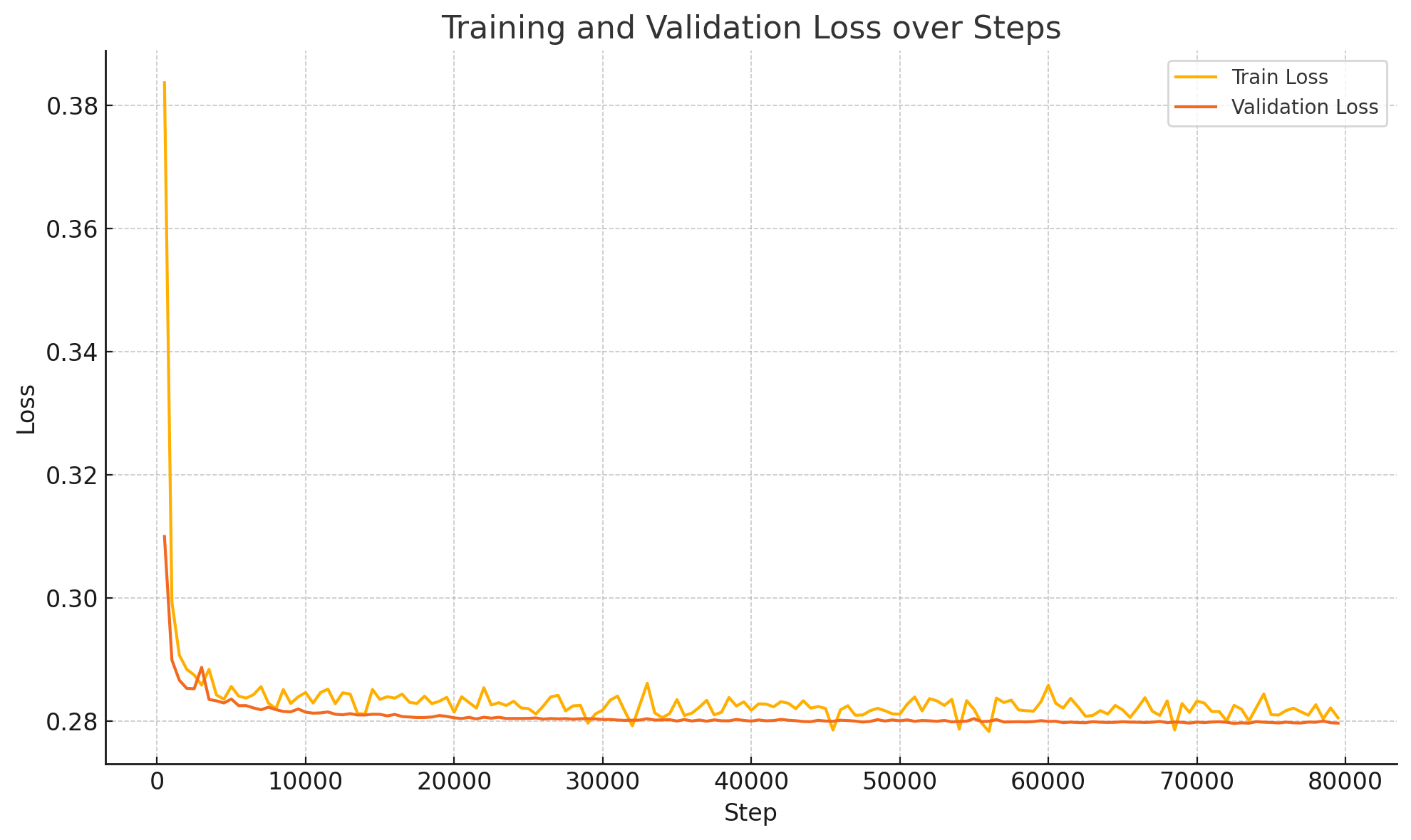
It seems like a reasonably healthy loss curve; perhaps there might be a bit of underfitting, as the model did most of its learning very early. It suggests we might only need 1M games or so to get most of the benefit, at least for this model. (Each step is a batch of 2048 positions; each game has around 24-25 positions).
Tuning the model
I put a quick little poll on Discord to ask how the first model would do. I secretly thought something around 45%, hoped for 55+%, and also believed there was a decent chance at < 10% vs HastyBot - due to screwing up something fundamental. I believe the 45-50% range won. I didn’t actually end up matching the very first model against HastyBot because there was something fundamentally wrong with it - I called it. It failed what I call “the ZYMURGY test”. With an opening rack of ZYMURGY, the bot should, well, play ZYMURGY for 120 pts. My bot thought GYM for 18 was better. So I called that a burner model and tried again.
The first broken model trained on spread difference after 5 turns. So for example, if the spread after playing a certain play is +30, and the spread 5 turns later is -75, the spread difference is -105; the network can learn that playing this move would lead to a spread difference of -105 in this one case, and hopefully averaging out over many cases there would be a learnable trend. But it failed badly. The loss curve, for example, had some shockingly low numbers, it was most likely because it kept trying to learn something tiny (I normalized the spread diff again with a tanh function) that hovered around zero with a lot of noise.
I then tried to just train on win/loss after 5 turns. This model did much better and I was able to run a match against HastyBot in which it won 43.7% of games. Slightly disappointing, but it was a start! The methodology is simple for this new bot that I dubbed “FastMLBot”:
- Generate 15 highest moves by equity (the metric that HastyBot uses)
- Evaluate all of them with the network and choose the highest
From there, it was just incremental addition of features and various changes that enabled the model to improve. Note that the tensor I describe above did not achieve its final form for a while. For the most part, adding new features kept improving it.
First good model
I added a few features:
- Added transposed board positions
- Added a validation set (it was only calculating losses on training before)
- Added our leave value in addition to our move score
Note that move score is already implicitly included in the spread, but removing it made the model perform worse. Often you have to just give ML models explicit features, to allow it to learn what really matters - board and timing considerations, in this case. We already know that score and leave matter. All that the previous static evaluator (HastyBot) cares about is score and leave.
I fixed a few bugs as well; my tensors did not always perfectly represent what I wanted them to represent. It is hard to debug giant vectors of 18,000 float32s, so Github Copilot I built a little visualizer tool (while we’re in this parenthetical, Copilot, ChatGPT, and Cline wrote a VAST amount of this code, with, of course, me to babysit them. It’s unreal how good they have gotten.)
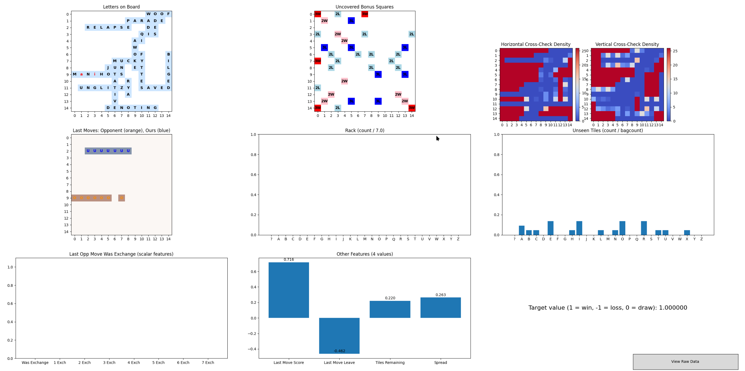
This visualizer helps us look at the raw streaming data going into the training loop. At a glance I can see if the board looks ok, if the tiles played look ok, and I can plug in other values into a calculator to see if it’s representing spread, etc correctly. I caught a significant number of bugs with this tool. So often, it wasn’t fully clear whether it was my bug fixes or feature improvements (or both) that would influence how a particular model run went.
I also sped up the inference part of the equation - that is, actually running the model. I initially converted the PyTorch model into ONNX and served it directly from my Go code. It was very slow, taking around 1 second to evaluate 15 moves. But this allowed me to run a few matches overnight for statistical significance. Actually, for the last couple of weeks, my CPU and graphics card have been busy running self-play sets, then training, then matches to see how well it did; the entire loop takes around 6-12 hours depending on how many games I do. I then found NVIDIA Triton, a model inference server - this can run models directly on my graphics card and is written in C++, does automatic batching, and so forth. I can get it to run approximately 800,000 inferences per minute - a big upgrade!
Anyway, after all of that, the first model that finally beat HastyBot is immortalized in these stats:
Games played: 31875
HastyBot wins: 15891.5 (49.856%)
HastyBot Mean Score: 446.5599  Stdev: 76.9168
FastMlBot Mean Score: 423.2252  Stdev: 67.2689
HastyBot Mean Bingos: 2.0627  Stdev: 1.0968
FastMlBot Mean Bingos: 2.0682  Stdev: 0.9830
HastyBot Mean Points Per Turn: 37.3685  Stdev: 6.3035
FastMlBot Mean Points Per Turn: 36.0960  Stdev: 7.6867
HastyBot went first: 15938.0 (50.002%)
Player who went first wins: 17987.5 (56.431%)
FastMLBot beat HastyBot 50.1% of the time! Woohoo! … :/
But can we do better?
Changing the training set a bit
Our training set consisted until now of millions of HastyBot vs HastyBot games. Again, with Gemini or o3’s help (I’m kind of an LLM himbo, the best models are mostly interchangeable in my head), I came up with what I call a Softmax bot. Let me first outline the problem, what I now call the JUT problem. If you’re playing a game of Scrabble, and you decide to open the game with the word JUT, you should put the U on the center star. This is just what people do; it’s the most defensive position as 1) vowels should not be placed directly next to 2LS squares if you can help it and 2) it doesn’t give your opponent easy access to the 2W lane. But my bot liked playing JUT in the other two positions, just barely. Why?
It never learned not to! HastyBot has a hard-coded hack for only the first move where it deducts a few fractions of a point for every play where a vowel is next to a 2LS square. So it doesn’t know not to do that. I tried playing bots that played randomly bad moves once in a while but they ended up in worse models. The trick is to make “once in a while” more mathematically rigorous. Using an exponential softmax formula - see Softmax function - you can suppress but not fully disable the bot from making bad moves. I created a bot with a “temperature” of 1 - the temperature controls the suppressive behavior of the function - and set the temperature to 0 below 60 tiles in the bag. Kind of handwavy numbers, like much of deep learning…
In any case, matching this softmax bot vs HastyBot created my best-performing training set yet. With this set, the next iterations of our FastMLBot learned how to position opening plays without having to add hacks. It also hopefully learned more about when lower equity plays can actually result in better outcomes. Changing that 60 to 0 (i.e. doing softmax for the whole game) resulted in a worse ML bot though. It all seems very experimental and I might try a temperature that slowly decreases to 0 with tiles remaining, just to see what happens.
As a side note, I never have any idea what to expect with these features / changes. It reminds me of all the stuff I would do for the endgame engine back in the day that would always end up slowing it down instead of speeding it up. Making Scrabble engines is hard.
This model resulted in a little improvement, now FastMLBot wins 50.25% of its games. Ok, that’s a little better!
What else can we do?
We added a representation of our last play on the board, as well as the opponent’s last play. The more features the better? Maybe it can learn to infer or defend better, or “visualize” hooks and lanes better, who knows? But this resulted in a FastMLBot that wins 50.6% of its games. Making some progress now!
Bogowin
We tried training on Bogowin as a target variable. Bogowin is essentially a table of win percentage, calculated through millions of self-play games. It’s a lookup table where the arguments are inputs are the number of tiles left in the bag and the current spread, and the output is an estimated win percentage. Macondo has its own Bogowin lookup table, and it is used whenever we do Monte Carlo simulations; it is the main parameter that we sort by at the end of a simulation.
An example of Bogowin (shown as Win % in the table below) for a typical Macondo position.
macondo> sim show
Play                Leave         Score    Win%            Equity
 1G NOUNA(L)        AY            18       57.81±0.84      -28.44±1.68
 K9 NOYAU           AN            18       57.59±0.90      -28.79±1.92
 1G ANNUA(L)        OY            18       57.46±0.84      -29.27±1.68
 1L (L)UNY          AANO          21       56.42±1.17      -31.53±2.35     ❌
N10 ANNOY           AU            25       54.23±2.39      -35.95±5.07     ❌
 1L (L)UNA          ANOY          12       53.70±2.53      -36.43±4.98     ❌
N10 ANYON           AU            25       53.11±3.01      -37.98±6.41     ❌
 1H ANNU(L)         AOY           15       51.50±3.67      -40.90±7.23     ❌
 1H NONY(L)         AAU           24       49.37±5.49      -44.58±11.06    ❌
 I8 (F)AUN          ANOY          11       48.60±5.79      -48.80±12.87    ❌
 G8 (G)UANAY        NO            15       48.01±5.93      -48.39±12.68    ❌
L10 ANYON           AU            19       47.73±6.16      -50.52±13.02    ❌
 2H NOYA(U)         ANU           16       47.56±5.06      -48.33±9.77     ❌
L10 ANNOY           AU            19       46.85±6.16      -52.68±13.54    ❌
 I8 (F)AUNA         NOY           12       46.45±6.10      -51.27±12.93    ❌
Iterations: 5254 (intervals are 99% confidence, ❌ marks plays cut off early)
Training with Bogowin as the target variable also resulted in a some bad results, but at the same time they were quite interesting. Let’s take a look:
Games played: 156888
HastyBot wins: 83533.5 (53.244%)
HastyBot Mean Score: 456.7695  Stdev: 73.5927
FastMlBot Mean Score: 400.8373  Stdev: 73.0475
HastyBot Mean Bingos: 2.0614  Stdev: 1.0645
FastMlBot Mean Bingos: 1.7964  Stdev: 1.0367
HastyBot Mean Points Per Turn: 36.2815  Stdev: 6.0308
FastMlBot Mean Points Per Turn: 32.9691  Stdev: 8.1514
HastyBot went first: 78444.0 (50.000%)
Player who went first wins: 87905.5 (56.031%)
FastMLBot wins 46.75% of its games against HastyBot, which isn’t great. But look at those average scores. FastMLBot is scoring a full bingo worth of points fewer than HastyBot every game, while still managing to beat it nearly half the time. It must be a very interesting bot to play against; perhaps it is playing a very restrictive/defensive style? Very interesting.
We then ran a longer number of games, 7.5M games (as opposed to 4-5 M games) and re-trained another model. We also ran a longer number of inference games so we can get the least margin of error that we can. This resulted in a 51% edge for FastMLBot over HastyBot. Not bad!
Changing the horizon
Our target variable to date has been whether we are winning or losing 5 plies after the play that we are evaluating. There was some speculation on Discord that perhaps 5 plies is too far to look ahead. Surely there would be a bunch of noise and maybe we should look more immediately ahead. So I tried using the same 7.5M game dataset but changed the game assembler code to calculate feature tensors with 3 and 4 plies as well:
| Horizon | FastMLBot Win Rate |
|---|---|
| 5 plies | 51.0 % |
| 4 plies | 50.7 % |
| 3 plies | 49.8 % |
This was a bit surprising to see. I think I expected a sort of bump around 5 plies and then fall-off in either direction. The main reason for this is that my Monte Carlo bot (BestBot, more on him later) has the best performance with 5-ply look ahead. It seemed to strike a good balance between lookahead and less noise. Scrabble is a very “noisy” game. Besides there being a huge amount of randomness in the tiles that you draw, there’s also a lot of randomness in how the plays you make affect future boards and your own chances to win. There are uncountable stories about making bad mistakes that directly lead to you winning the game. This is one of the many reasons building a neural network for Scrabble is difficult.
So I went ahead and changed lookahead to 50 plies (which has the effect of looking to the end of the game) and got the best performing model yet!
And now, for the best model…. (so far)
Games played: 255626
HastyBot wins: 123589.5 (48.348%)
HastyBot Mean Score: 436.4643  Stdev: 70.1158
FastMlBot Mean Score: 425.7528  Stdev: 61.0820
HastyBot Mean Bingos: 2.0229  Stdev: 1.0709
FastMlBot Mean Bingos: 1.9990  Stdev: 0.9579
HastyBot Mean Points Per Turn: 37.4571  Stdev: 6.4241
FastMlBot Mean Points Per Turn: 36.7565  Stdev: 6.9454
HastyBot went first: 127813.0 (50.000%)
Player who went first wins: 143352.5 (56.079%)
FastMLBot wins 51.7% of its games against HastyBot. Yay!
What’s the big deal?
A little primer on HastyBot. Since the 1980s, it’s been thought that Scrabble is very largely a game of scores and leaves. I wrote about this in this article, in which I assert that Scrabble is not a solved game, and that Scrabble is NOT just a game of scores and leaves. HastyBot, our most played bot on Woogles, uses a very simple algorithm to choose its top move; it generates all moves, and picks the move with the best combination of scores and leave. Leaves are chosen through literally billions of games of self-play and they’re the best values that we know of. The algorithm takes microseconds to run for any given position.
With such a simple bot, it will mess up endgames, it will open up triple-triple lanes while ahead, it will not be able to sniff out opponent’s setups, and it will make all sorts of what we think of as terrible plays, and yet, I would put money on maybe a few dozen players in the entire world to beat it in a 100-game series. It’s undeniable that being perfect at finding every available play and having a good leave calculation methodology results in a bot that’s very hard to beat.
Static evaluator
The algorithm that this bot uses is also known as “the static evaluator”. It does a quick, static evaluation of a board position. We also have a better bot, appropriately named “BestBot”, which uses Monte Carlo simulations, perfect endgame and pre-endgame solving, and more. You can read more about it here. But behind BestBot’s Monte Carlo simulations is the good old static evaluator, HastyBot. Every rollout must use the static evaluator to find the “best move”. And as we’ve established, HastyBot’s top move in any given position can be all sorts of wrong. Indeed, many of BestBot’s mistakes come from situations such as closed boards where its static evaluator thinks that your opponent will incorrectly open a lane, and thus it doesn’t bother to open another lane even though it is behind. This is just one example of situations that it gets wrong.
Still, with all that firepower, BestBot can beat HastyBot about 59 to 60% of the time in a long series. It can take minutes to find its top move, though. We at Woogles think it’s worth it, even though it’s literally millions of times slower than HastyBot, to have the best known Scrabble engine as a sparring partner on our site. Current North American champion Mack Meller told us that during his heartstopping best-of-5 series for the championship, he was down 0-2 and close to losing the third game when he thought, “What would BestBot do in this situation?” and turned it around from there. So I’ll take a tiny bit of credit for that win 😅.
In any case, having a significant improvement on our static evaluator opens the door to future improvements to BestBot, as well as hopefully starts to teach us more about Scrabble. I agree that 51.7% is a fairly modest improvement, but I believe this is just the beginning. Casino edges are often smaller than that and we have seen those ridiculous fountains at the Bellagio :)
Replacing BestBot’s static evaluator with a neural network could unlock major advances. This is essentially the approach AlphaGo took with Go: its Monte Carlo Tree Search was guided by a neural network-based evaluator, refined over several iterations. The result was a truly superhuman, virtually unbeatable bot.
We don’t think there can ever be such a thing as an unbeatable bot in Scrabble, there’s simply too much randomness. The best player in the world loses 25% of his games, and closer to 50% against other top players. But it would be fun to make the best bot that we can. I am mostly excited about what it can teach us about the game that we don’t yet fully understand, and excited about driving the quality of play up worldwide.
What’s next?
There are many improvements we can make. Here I list a few ideas:
- Continue trying other combinations of parameters and features. We can add more board and timing features, we can explicitly add bingo lanes (instead of having the network deduce them from the cross-checks). We can try different learning rates (it seems to be settling down pretty quickly), different softmax parameters.
- We can add more “heads” or things that the network predicts. Besides providing interesting data - we can try predicting next move score, next move bingo percentage, and so on - adding more heads typically stabilizes and makes the network a bit better, even if we don’t end up using the predictions.
- We can change the training set to be BestBot vs BestBot games, or BestBot vs Humans, and add in a bunch of expert games from cross-tables / other places. I think this would drive the quality of the network up as well. The main issue is the time it takes to collect this data. I may ask the community to help me crowd-source more games; I will work on a
volunteercommand in Macondo that allows users to donate their computing power to self-play a bunch of BestBot games. - We can try a NNUE architecture. NNUEs are super fast neural networks that can run on CPUs. Right now, our current model requires a GPU if it doesn’t want to be dog slow. NNUEs revolutionized computer chess; Stockfish with NNUE is the strongest player in the planet now.
- We can replace BestBot’s static evaluator with this new model. This seems like an obvious thing to try - but we’ll need to make some changes to speed it up a bit more, as some Monte Carlo simulations involve many, many thousands of static evaluations.
Can I try it?
The code is available in the Macondo GitHub page. See the pytorch directory for training code. You can run the model locally (use the mleval command after generating plays) and it will be kind of slow unless you figure out how to set up Triton and you have a good graphics card. I also have not created a model version for the CSW24 lexicon yet. All of these models and results are for the North American NWL23 lexicon. I expect the model to do well in CSW too, but slightly less so; HastyBot is a bit better at CSW than at NWL, comparatively.
I will try to release the bot for you to play against on Woogles as well (what should we name it? BrainBot? MycroftAKAMike? Robotron 2000?). Give us a few days/weeks to get it all ready. There’s also the matter of training it on other lexica/letter distributions. A lot of it is currently hard-coded for English.
Here are a few sample positions that I found interesting:
Position #1
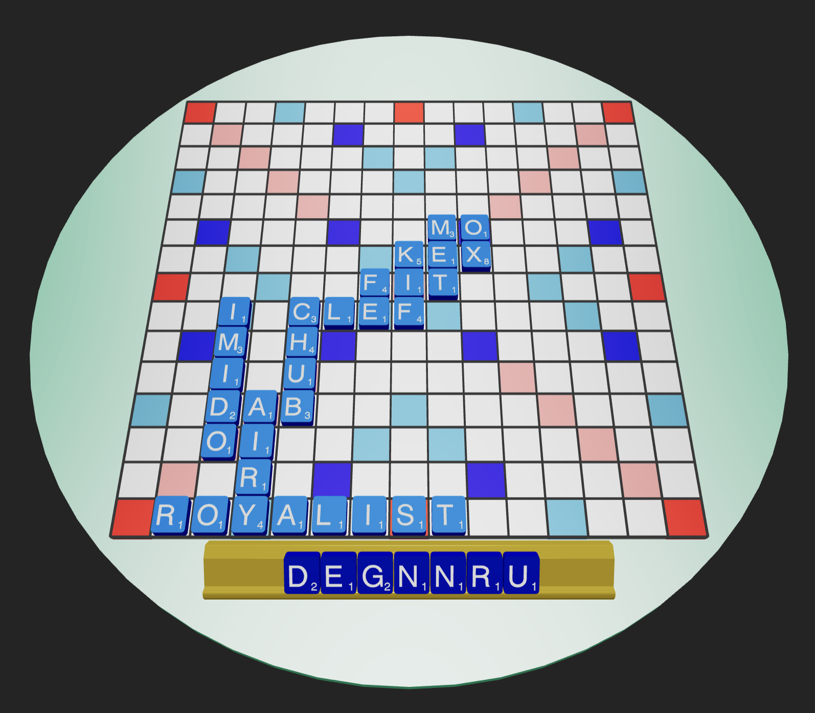
We are up 139-107 in this position, with 55 tiles in the bag.
In this position, the static evaluator prefers the play 5J GUNNED, forming GOX horizontally, on top of the OX. This play opens several bingo lanes on a fairly tight board while the player is ahead, including a potentially dangerous triple lane.
However, the neural network in this blog post prefers 5J DUNG in the same spot, making it tighter for our opponent and keeping a better leave for ourselves. BestBot prefers 5J GNU by a little bit more, but both plays are better than 5J GUNNED.
If this was an intermediate position that was reached by a Monte Carlo simulation, the static evaluator would always choose GUNNED here with this rack, thus potentially misevaluating the original play that is being examined.
Position #2
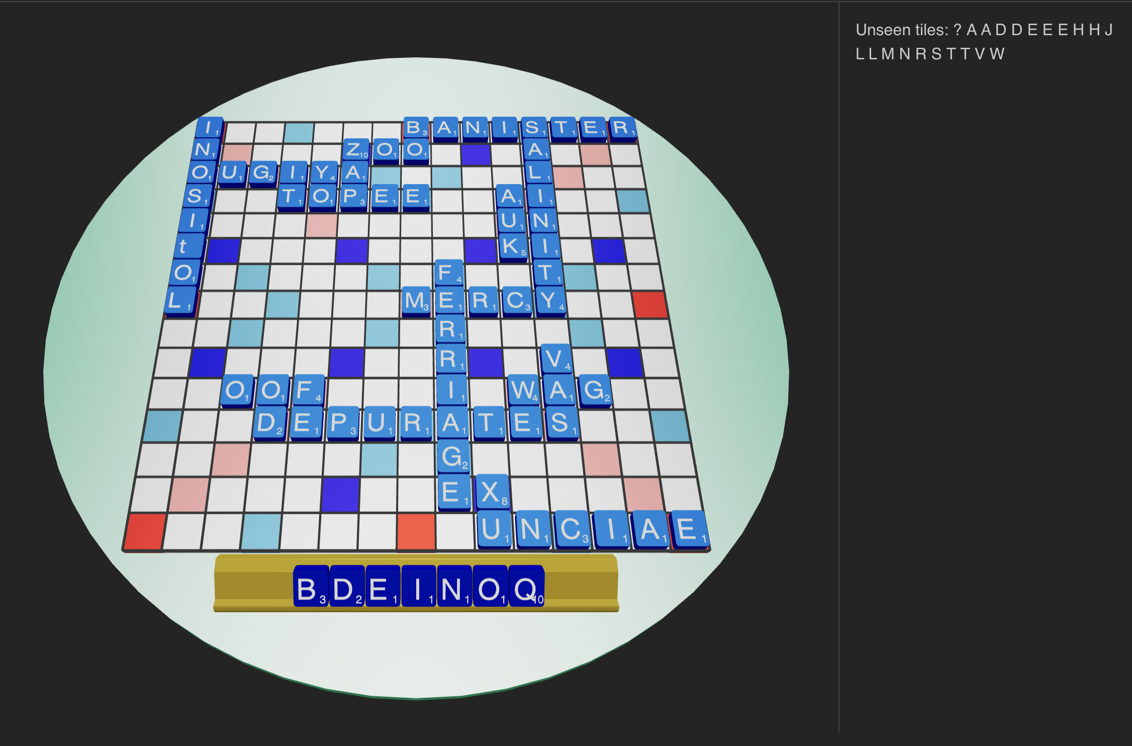
In this late game position, we are down 383-428 and the bag has just 14 tiles in it. The static evaluator prefers the play 13A BONED, making ODE and FED vertically. This isn’t a great play; it blocks a weak bingo lane making a whole bunch of _OOF plays (HOOF/LOOF/ROOF/WOOF/etc), and it leaves the Q on our rack without a good place to put it. Our opponent’s next play will likely involve playing in the bottom right quadrant, trying to mess up the WAGE hook and shutting down the board. We’re often not in a good position to win this game after BONED, despite its high score.
The neural network picks the BestBot-preferred play here, G11 Q(U)OD, through the U in DEPURATES, even though it ranks #13 in the list of static plays. It sheds the bad Q, turns over a couple more tiles for the blank, sets up a hard-to-block, somewhat desperate lane for an S or blank that we don’t yet have – but it’s ok to do this when we’re in this position, where we’re in trouble! This would leave the opponent several annoying bingo lanes to deal with. It’s great that it figured this out.
There’s also a very interesting play that the neural network ranks right below QUOD here: just dumping the Q at M14 to make QI (on top of the I in UNCIAE). This sets up OBIA/QI next turn for 34 points and it keeps a decent leave. It won’t result in a bingo often, and it’s not a great play either, but it’s not the kind of play the static evaluator would make. I can kinda dig it.
Thanks for reading this far!
If you’re interested in using neural networks to “solve Scrabble”, shoot me an email or join our Woogles Discord. I think we’re starting to make some good progress!